Near Real-time Analytics, Operational Data Store, Lakehouse Analytics, and Observability Data Lake are gaining popularity, and they share the same underlying foundation - a fast OLAP engine such as ClickHouse, StarRocks, Trino, e6data. This article studies a simple scenario in which the very-easy-to-write queries can choke the most powerful engine even StarRocks or ClickHouse. We also want to share a few design patterns which can be effectively improve QPS by 7~15x without throwing more hardware into the game.
- Do More with Less: By reducing I/O amplification, we’re getting more performance per dollar out of the existing hardware.
- Predictability: Full table scans cause “noisy neighbor” issues. The optimization doesn’t just make one query faster; it made the whole system more stable for everyone.
- Knowing where to tap: At Stateful Data, we believe that ‘big data’ shouldn’t mean ‘expensive data’. Effective schema & query design beats throwing hardware at the problem every time.

Table of contents
Why StarRocks and ClickHouse?
TP (OLTP) databases go nuts whenever full table scans happen, adding too many indices significantly increases the write-lantency and vaccum/compact overhead. Snowflake and Databricks SQL Serverless are popular but they are quite expensive and can’t handle decent concurrent queries. Trino and other DataFusion/Velox-based engines are catching up. Pinot and Druid have their different tradeoffs for the above 4 use cases. StarRocks/Doris is widely used in e-commerce and ODS scenarios with sub-second latency & 100+ concurrency. ClickHouse has proven success in handling large volume of logs and events. Both StarRocks and ClickHouse have the compute nodes implemented in C++ with extensive optimizations for SIMD vectorization. Those nodes are mainly live, with warmed-up caches, and ready to serve queries immediately.
https://www.ssp.sh/blog/starrocks-lakehouse-native-joins/ is a good summary of why.
https://www.onehouse.ai/blog/apache-spark-vs-clickhouse-vs-presto-vs-starrocks-vs-trino-comparing-analytics-engines is a great comparison.
Problem
When the data model was designed and initial benchmark was measured, the team probably has only 50M records loaded with 2~3 concurrent queries, so everything went just fine. Once this is deployed to production and after 5+ years of historical data are backfilled, the query latency alerts keep flashing, and the QPS don’t visibly improve even if you add a bunch of compute nodes.
Well, we can pop the following into LLM and see what they suggest.
Prompt
We have a huge amount (1B~100B records across 5+ years) of transaction/transfer data in an OLAP database.
create table transfers_clustered_native_v1 (
  -- starrocks syntax
  transaction_time timestamp,
  transaction_hash string,
  transaction_batch_hash string,
  from_address string,
  to_address string,
  type string,
  currency string,
  amount decial(38,12),
  properties json,  -- a whole bunch of K,V
  INDEX idx__to_address (to_address) USING BITMAP,
  INDEX idx__tx_hash (transaction_hash) USING BITMAP
 )
DUPLICATE KEY (from_address, to_address, transaction_time)
PARTITION BY date_trunc('month', transaction_time)
DISTRIBUTE BY HASH (transaction_hash)
PROPERTIES("bloom_filter_columns" = "transaction_hash,from_address,to_address");

CREATE TABLE transfers_clustered_native_v1
(
    -- clickhouse syntax
    transaction_time DateTime64(3),
    transaction_hash String,
    transaction_batch_hash String,
    from_address String,
    to_address String,
    type LowCardinality(String),
    currency LowCardinality(String),
    amount Decimal128(12),
    properties Json,  -- or String before v25

    INDEX bloom__from_address from_address TYPE bloom_filter(0.01),
    INDEX bloom__to_address to_address TYPE bloom_filter(0.01),
    INDEX bloom__tx_hash transaction_hash TYPE bloom_filter(0.001)
)
ENGINE = SharedMergeTree('/clickhouse/tables/{uuid}/{shard}', '{replica}')
PARTITION BY toYYYYMM(transaction_time)
ORDER BY (from_address, to_address, transaction_time);
There are several microservices and BI dashboards which query this table with quite a lot of concurrent queries with 3 of the most popular shapes like below.
SELECT * FROM db.transfers_clustered_native_v1
WHERE from_address = ?   -- the cardinality of from_address and to_address is high
ORDER BY transaction_time DESC LIMIT 200;

SELECT * FROM db.transfers_clustered_native_v1
WHERE from_address = ? OR to_address = ?  -- this query shape has the highest frequency
ORDER BY transaction_time DESC LIMIT 200;

SELECT * FROM db.transfers_clustered_native_v1
WHERE transaction_hash = ?;  -- or transaction_hahs in (?, ?, ?)
The throughput (QPS) is supposed to go as high as 100~500, does GPT/Claude/Gemini detect any obvious problems of this design? What can be the mitigation options?
BTW, if OLAP databases are not the right choice, is there any OLTP (MongoDB or Aurora) or HTAP database can get the job properly done?
Root Cause
What do AIs say
GPT may say this is a problem that TP query patterns spill into an AP database. But
| the mistake is thinking the choice is | While the real choice is |
|---|---|
| OLAP vs OLTP | Monolithic OLAP record layout vs Multiple layouts |
- Sort keys are misaligned with the hot queries’ predicate/filter
Parition By (f1) is the coarse-grain ordering, Order By (f2, f3) determines the fine-grain, but f1 has a higher precedence than f2, while filter against f3 without f1 and/or f2 still leads to full table scan
ORpredicate is the worst possible shape at scale
This is very often a mistake overlooked/ignored by developers
-
Partitioning by
timedoes not help the hot queries -
Distribution by
transaction_hashis optimizing the least-frequent query shape -
SELECT *+ JSON at high QPS can be deadly -
Secondary indexes have more overhead than benefit
Both Claude & Gemini also point out the I/O (and thread pool) saturation caused by scan too many data files yet return a few records.
Highest Truth is Simplest
Even though StarRocks and ClickHouse are very fast in terms of querying large amount of data, once there are 10 full table scan operations going through hundreds of thousands of files (or tablets), the cluster slow down dramatically. Then a lot of queries are put into the wait queue, and the overall query latency shoot up significantly. This behavior is even worse in Snowflake and Databricks.
So fundamentally, we have to find an effective way to seriously reduce full table scans. In the recommended solution section, we will explain how to reduce the scan range in stead of pure number of concurrent scans.
Database is not a blackbox, the query shapes need to be aligned with the physical data model, vibe coding needs to be guardrailed by precise DOs and DON’Ts.
Solution
We can’t simply leverage a single sort order to satisfy different predicate/filter patterns, therefore we have to make some serious tradeoffs with reasonable estimations. The Stateful Data team strongly oppose the notion that developers don’t need to understand (or to ask AI about) the database internals; if we put effort to tuning the QPS and latency, 80% energy should be focusing on query logic & application code, while only 20% goes to database parameters or right-sizing.
1. Iterative Temporal Reverse Scan
For the most recent records logic ORDER BY transaction_time DESC LIMIT 200, it is very very very wasteful to first
scan 5+ years of partitions, fetch all the records for a certain from_address and/or to_address, then discard most of the
old ones.
Materialized View to Prune
A monthly pre-aggregated table or materialized view plays a key role here:
CREATE TABLE mv_monthly_address_stats (
    month_begin_date date,
    next_month_begin_date date,
    address string,
    -- stats
    num_of_transactions__from int,
    num_of_transactions__to int,
    min_transaction_time timestamp,
    max_transaction_time timestamp
)
PRIMARY KEY (address, month_begin_date)
DISTRIBUTED BY HASH (address)
Two Query Phases
First use the mv_monthly_address_stats to conduct coarse-grain pruning for a given address:
SELECT month_begin_date, num_of_transactions__from, num_of_transactions__to
FROM db.mv_monthly_address_stats
WHERE month_begin_date >= ? AND month_begin_date <?
  AND address = ?
ORDER BY month_begin_date DESC
Let’s go over the most recent 24 months first. This kind of query is super quick because the predicates are well covered by the sort order already. StarRocks can respond to hundreds of such quick queries concurrently.
Then the application/service logic (in Java/Go/Python) iterates the result set to find
which particular months are worth scanning.
- The iterator stops once enough transactions are found. Let’s say that it determines that 5 months need to be scanned. Then 5 queries will be sent to the actual workers described in the “Scatter and Gather” section below.
- If only 2 months contain the qualified records but still less than 200, the iterator will iterate on
mv_monthly_address_statsagain with the previous 24 months. In the mean while, 2 scan queries are sent to the actual workers.
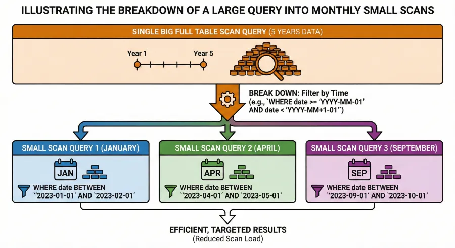
This step drastically reduces the wasteful scans. If iterator fires 5 queries for FEB, APR, SEP, OCT, DEC, then only 5 partitions will be scanned by 5 light-weight queries (any other monthly partitions won’t be scanned at all).
SELECT f1, f2, f3 , f4 FROM db.transfers_clustered_native_v1
WHERE transaction_time >= {{month_begin_date}} and transaction_time < {{next_month_begin_date}}
  AND (from_address = {{ the_address }} OR to_address = {{ the_address }})
2. Scatter and Gather
Each scan query has the temporal predicate which is perfectly aligned with a single partitio bondary, so we can concurrently execute many queries without exhausting the I/O bandwidth.
At the iterator level, we may set a limit for 300 concurrent queries before queuing kicks in. For a given address, we allow up to 3
concurrent scan queries.
In the above example, the iterator sends 5 scan queries to the workers, 3 of them get executed immediately in parallel. Once 1 of these 3 workers finishes, the 4th scan query starts. All the results are accumuated by a “gather” worker. Once all 5 scan queries are done, the result is sorted again and then returned to the application/service.
This is the typical scatter-gather pattern in distributed search index architecture. The total number of concurrent queries in StarRocks actually increase, but these queries are much more efficient especially I/O wise, so that they all finish quickly and yield the I/O bandwidth and thread pool back to the next query.
The overall QPS improves visibly with this trick.
3. Trade Space for Speed
Since the layout is tailored to from_address only, we have to do something for to_address. This is where benchmark with production
data volume is important. We have three options:
- Leverage a BITMAP INDEX for the
to_address. The assumption is that its cardinality within a single month is OK for BITMAP index. - Create another duplicate but having
DUPLICATE KEY (to_address, transaction_time), or adddirectionto duplicate the TX so that theFROM_ADDRESScan play double roles.
| HASH | FROM_ADDRESS | DIRECTION | TO_ADDRESS | AMOUNT | … |
|---|---|---|---|---|---|
| 5AUeNPgqxNyunQaWo3nv4 | 0x12345678 | SELL | 0x78901234 | -0.0002175 | … |
| 5AUeNPgqxNyunQaWo3nv4 | 0x78901234 | BUY | 0x12345678 | 0.0002175 | … |
This approach can accelerate WHERE (from_address = ? OR to_address = ?) queries, however, it makes all the other query shapes
more complicated. Also in the real world, the table have many fields, and the JSON field is quite big, so visible overhead here.
- Create a LEAN table (which acts like an covering index) just for the speedy lookup of
to_address. The main table has the unique key(from_address, transaction_time), while the lean table looks like:
create table transfers_clustered_native_v1__by__to_address (
  transaction_time timestamp,
  transaction_hash string,
  transaction_batch_hash string,
  from_address string,
  to_address string,
  type string,
  currency string,
  amount decial(38,12)
  // properties json,  -- exclude any big/fat fields
)
DUPLICATE KEY (to_address, transaction_time)
PARTITION BY date_trunc('month', transaction_time)
DISTRIBUTE BY HASH (to_address)
The scan query will be more complicated:
SELECT f1, f2, f3 FROM db.transfers_clustered_native_v1
WHERE transaction_time >= {{ month_begin_date }} AND transaction_time < {{ next_month_begin_date }}
  AND from_address = ?
UNION ALL
SELECT a.f1, a.f2, a.f3 FROM transfers_clustered_native_v1 a JOIN transfers_clustered_native_v1__by__to_address b
ON a.from_address = b.from_address AND a.transaction_time = b.transaction_time
WHERE a.transaction_time >= {{ month_begin_date }} AND a.transaction_time < {{ next_month_begin_date }}
  AND b.transaction_time >= {{ month_begin_date }} AND b.transaction_time < {{ next_month_begin_date }}
  AND b.to_address = ?
For transaction_hash lookups, we can create another table ordered by transaction_hash, or we can measure how effective
the bitmap index and bloom filter are.
4. What Else
In the original DDL, DUPLICATE KEY (from_address, to_address, transaction_time) is suboptimal, we should remove to_address
from the KEY.
Since the main table is optimized for filters based on from_address, the hash distribution does not have to use from_address
anymore. It is OK to use transaction_hash to compensate transacation_hash lookups. This is a minor tweak, yet both choices
are OK, the query shape frequency really matters here.
If the string of address is very long, such as 5AUeNPgqxNyunQaWo3nn3Umq5p7RhVw4eG1TyDraSYTJ2SmnFpTUhy1BhdKucmDNsb46LNuiW7CEHKx9NSGQhwMN, it can make a big difference when
from_address_hash and to_address_hash is used instead:
- https://docs.starrocks.io/docs/sql-reference/sql-functions/hash-functions/xx_hash3_64/
- https://docs.databricks.com/aws/en/sql/language-manual/functions/xxhash64
- https://trino.io/docs/current/functions/binary.html (xxhash64)
- https://duckdb.org/docs/stable/sql/functions/utility#hashvalue
The Trade-offs
The first and foremost tradeoff is to implement more a complex scatter-gather coordinator with a monthly aggregate table.
The second one is to respect the limitation of layout (partition & sort order), trading space for speed instead of blindly dumping all kinds of query shapes to the single table layout.
The third one is “size matters”: lean table and bigint hash value for address are worth exploring.
Last but not least, profiling the data, understanding the histograms and query shape frequency, test the hash collision against the production data, and seriously leverage the “query profile” tool provided by StarRocks and ClickHouse to detect and understand the slow query shapes which hog the resources and conduct inefficient/wasteful operations.
The above analysis and tuning patterns are not limited to ClickHouse and StarRocks. Especially those suboptimal or abusive the above optimizations, we have observed 7~15x query performance improvement. query shapes (and oversimplified designs) are frequently seen in Snowflake, Databricks and others as well. After applying
Brute force scanning is possible in Netzza, Hadoop, Snowflake, Databricks, ClickHouse, … however it destroys the overall system throughput, and the cloud bills add up crazily if many full table scans are issued by BI or AI agents. If developers can pay attention to the basic database pinciples and restrictions, we believe that AI can help generate the software code, query, and table structure to strike a reasonable balance for near real-time analytics with pretty decent concurrency.
- https://medium.com/starrocks-engineering/detailed-comparison-between-starrocks-and-apache-doris-81ddd34be527
- https://www.databend.com/databend-vs-starrocks
- https://medium.com/@indomitability/why-starrocks-is-better-than-apache-pinot-for-customer-facing-analytics-170757a06a1c
- https://youtu.be/Wl25FFBJPZA?t=668
- https://clickhouse.com/blog/alexey-p99-2025-rust-in-clickhouse
- https://www.alibabacloud.com/en/developer/a/e-mapreduce/emr-starrocks-data-lake-analysis